Routing Strategies in WSN
November 3, 2016
Categorised in: Data Communicaiton & Wireless Sensor Networks
Aim to make communication more efficient
Trade-off between routing overhead and data transmission cost
Strategies incur differing levels of communication and storage overhead
Hybrid approaches are possible
Stateless Routing
Nodes maintain no routing information
Flooding
–Messages rebroadcast to neighbours
Gossiping
–Messages rebroadcast to neighbours, probability <1
Geographic
–Need to know direction to destination
Epidemic
–Pairwise exchange of messages between carriers
–Copes with temporary network partition
–No routing state, but message buffering infeasible in WSNs
Proactive and Reactive Routing
Proactive routing
–Routes created and maintained in advance
–Low latency, high resource demand
–Does not scale to large networks
Reactive routing
–Routes created and cached as required
–High latency, lower resource demand
Data-centric Routing
Routing application data rather than packets
Node identities unknown to users
Data naming and labelling
Users express interests in named data, protocol sets up data flows
Combines routing and distributed data management
Data aggregated and summarised in flows
Well suited to WSN paradigm
Flooding
Used in data delivery or route discovery
Very simple algorithm, implicit multicast
Observed results surprisingly complex
–Stragglers, Backward Links, Long Links, Clustering
Last 5% of nodes take as much time as preceding 95%, independent of radio power
Some nodes will never receive the message
Redundant communications waste energy
Creates weird routes
Some nodes not getting the message is OK in a WSN, the high energy cost is not
Location-Based Routing Protocols
Nodes’ positions are exploited to route data
–Sensor nodes are addressed by means of their locations
–Distance can be estimated on the basis of incoming signal strengths
Protocols:
- Geographic Adaptive Fidelity
- Geographic and Energy Aware Routing
- MFR, DIR and GEDIR
- The Greedy Other Adaptive Face Routing
- SPAN
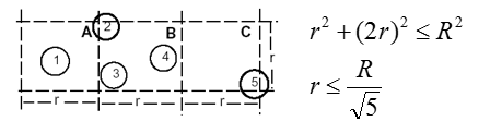
Geographic Adaptive Fidelity
Core idea
–Turn off a node if it is equivalent from a routing perspective
–Adaptively adjust routing fidelity use node deployment density
Determine routing equivalence

What’s fidelity
–Uninterrupted connectivity between communicating nodes
Use GPS information to decide virtual grid ID
3-state transition
- Discovery (Td)
- Active (Ta)
- Sleep (Ts)
Node ranking
–Active node wins
–High energy node wins
Adapting to mobility
–With GPS information

Motivation:
–Reduce overhead of interest and low rate data flooding in directed diffusion
Basic ideas:
- Leverage geographical information to restrict flooding, and recursively disseminate data inside the target region.
- Extend overall network lifetime using local techniques to balance energy usage
- Reuse routing information across multiple user queries.
Geographic and Energy Aware Routing
Forward the packets towards the target region:
- Greedy mode: minimizing cost function (f=mix function of distance and energy)
- Route around “communication holes” with energy aware neighbor estimation
Disseminate the packet within the target region:
Geographic Recursive Forwarding
- recursively re-send packets to sub-regions of the original geographic region
- Each node has a learned cost (historical cost) and an estimated cost (present state cost) to decide the next forwarding node
GEOGRAPHIC ROUTING
GPSR: Greedy Perimeter Stateless Routing for Wireless Networks
A sensor net consists of hundreds or thousands of nodes
- Scalability is the issue
- Existing ad hoc net protocols, e.g., DSR, AODV, ZRP, require nodes to cache e2e route
- information
- Dynamic topology changes
- Mobility
Reduce caching overhead
- Hierarchical routing is usually based on well defined, rarely changing administrative boundaries
- Geographic routing
- Use location for routing
Scalability metrics
Routing protocol msg cost
–How many control packets sent?
Per node state
–How much storage per node is required?
E2E packet delivery success rate
Assumptions
Every node knows its location
- Positioning devices like GPS
- Localization
A source can get the location of the destination
802.11 MAC
Link bidirectionality
Geographic Routing: Greedy Routing

Benefits of GF
A node only needs to remember the location info of one-hop neighbors
Routing decisions can be dynamically made
Greedy Forwarding does NOT always work

If the network is dense enough that each interior node has a neighbor in every 2/3 angular sector, GF will always succeed
Energy-Aware Routing
Maximise network lifetime (no accepted definition)
Communication is the most expensive activity
Possible goals include:
- Shortest-hop (fewest nodes involved)
- Lowest energy route
- Route via highest available energy
- Distribute energy burden evenly
- Lowest routing overhead
Distributed algorithms cost energy
Changing component state costs energy
A destination-initiated reactive protocol
It maintains a set of paths
Choosing paths by means of certain probability depending on how low the energy consumption is
Setup Phase

Data Communication Phase

Attribute-based routing
Data-centric approach:
–Not interested in routing to a particular node or a particular location
–Nodes desiring some information need to find nodes that have that information
Attribute-value event record, and associated query
| type | animal |
| instance | horse |
| location | 35,57 |
| time | 1:07:13 |
| type | animal |
| instance | horse |
| location | 0,100,100,200 |
Directed diffusion
Sinks: nodes requesting information
Sources: nodes generating information
Interests: records indicating
–A desire for certain types of information
–Frequency with which information desired
Key assumption:
–Persistence of interests
Approach:
–Learn good paths between sources and sinks
–Amortize the cost of finding the paths over period of use
Diffusion of interests and gradients
Interests diffuse from the sinks through the sensor network
Nodes track unexpired interests
Each node maintains an interest cache
Each cache entry has a gradient
–Derived from the frequency with which a sink requests repeated data about an interest
–Sink can modify gradients (increase or decrease) depending on response from neighbors
Flat Routing
Each node plays the same role
Data-centric routing
–Due to not feasible to assign a global id to each node
–Save energy through data negotiation and elimination of redundant data
Protocols
–Sensor Protocols for Information via Negotiation (SPIN)
–Directed diffusion (DD)
–Rumor routing
–Minimum Cost Forwarding Algorithm (MCFA)
–Gradient-based routing (GBR)
–Information-driven sensor querying/Constrained anisotropic diffusion routing (IDSQ/CADR)
–COUGAR
–ACQUIRE
–Energy-Aware Routing
–Routing protocols with random walks
Sensor protocols for information via negotiation (SPIN)
Features
Negotiation
–to operate efficiently and to conserve energy
–using a meta-data
Resource adaptation
–To extend the operating lifetime of the system
–monitoring their own energy resources
SPIN Message
- ADV – new data advertisement
- REQ – request for ADV data
- DATA – actual data message
- ADV, REQ messages contain only meta-data
Operation process

Resource adaptive algorithm
When energy is plentiful
–Communicate using the 3-stage handshake protocol
When energy is approaching a low-energy threshold
–If a node receives ADV, it does not send out REQ
–Energy is reserved to sensing the event
Advantage
Simplicity
–Each node performs little decision making when it receives new data
–Need not forwarding table
Robust to topology change
Drawback
Large overhead
–Data broadcasting
TOPOLOGY CONTROL Motivations
A typical characteristic of wireless sensor networks
–deploying many nodes in a small area
- ensure sufficient coverage of an area, or
- protect against node failures
Networks can be too dense: too many nodes in close (radio) vicinity
In a very dense networks, too many nodes
–Too many collisions
–Too complex operation for a MAC protocol
–Too many paths to be chosen from for a routing protocol, …
Topology control: Make topology less complex
Topology: Which node is able/allowed to communicate with which other nodes
Topology control needs to maintain invariants, e.g., connectivity
Options for topology control

Pratik Kataria is currently learning Springboot and Hibernate.
Technologies known and worked on: C/C++, Java, Python, JavaScript, HTML, CSS, WordPress, Angular, Ionic, MongoDB, SQL and Android.
Softwares known and worked on: Adobe Photoshop, Adobe Illustrator and Adobe After Effects.